Excel 2010 - Basics

A Few Basics

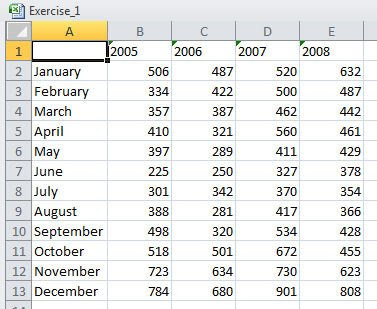
Before moving onto the more advanced features of Excel it is always good practice to run through a few basics to see if there are any changes in the general function of the program. I will do a few simple calculations and produce a chart in the same worksheet to show the results.

Having opened Excel I will type January in the cell A2 (I will use the convention of showing cells and formulas in bold i.e. =Sum(A1:A2)). Hit Return and the cell below will be selected. Click on January/A2 again, place the cursor in the bottom right corner of the thick border and drag it down to December, Excel will fill in the months. The same principle applies to any logical sequence, if I type A1; Return, and drag, it will fill in A2, A3, Etc. It also works laterally in rows but not with whole numbers.

Click B2, and type in the formula bar, ‘2005 and hit Return. The apostrophe before the year 2005 will mark the date as a ‘number stored as text’ and not as a number. Otherwise, 2005 as a number at the top of a list of numeric values would be included in any calculations later.

With B2 selected, drag it across to E1 ending in 2008. Three of the last four months in the A column exceed the standard size width of the columns. This can be adjusted manually but, to save time and be more precise, double click the line at the top of the columns separating A & B.

After keying in the numbers shown with B14 selected, click Auto Sum in the Editing Group. Excel will try to determine, in this case rightly, what sum you’re trying to do. It came up with the obvious formula =SUM(B2:B13). Which are B2+B3+B4 Etc.

Drag the bottom right corner of B14 across to E14 and the missing three totals will be added. Check the totals by clicking on them individually and look at the formula bar i.e. with D14 selected it reads =SUM(D2:D13).

With all four totals selected, right click and open Format Cells. On the Number Tab select Currency, 2 Decimal places and the Symbol £.

Select the four headings 2005 to 2008 and, holding the Ctrl key, select the four totals, on the Insert Tab Click Column from the Charts Group. From the Type Group change the chart type to suit your preference.

With the chart selected from Chart Tools > Design > Chart Styles choose one of the styles. In the table click, to select, the Vertical (Value) Axis, right click and open Format Axis. On the Axis Options change the Minimum setting from Auto 0.0 to Fixed 3000.0 and the Maximum from Auto to Fixed 6500.0 (charts will be covered in depth later)